Bayesian Optimization, Part 2: Acquisition Functions

This post continues our discussion on BayesOpt. This is part-2 of a two-part series. Now we take a look at the other pillar BayesOpt rests on: acquisition functions. My goal is to provide a flavor by looking at a few of them. I’ll go into depth for a couple; this would help us appreciate the role of GPs in conveniently calculating acquisition values. For the rest I’ll provide an overview.

• Acquisition Functions
  • Probability of Improvement
  • Expected Improvement
  • Predictive Entropy Search
  • Max-value Entropy Search
• Minimal Code for BayesOpt
• Summary, a Pet Peeve and Learning Resources
• References

Acquisition Functions

Note:

• Change in notation: \(x^*\) and \(y^*\) would refer to the current maxima (or minima) in this section.
• For brevity, we’ll denote an acquisition function by \(\alpha\).
• We’ll refer to the output’s Gaussian parameters at an input \(x\) as \(\mu(x)\) and \(\sigma(x)\).
• We’ll refer to the Normal distribution with \(0\) mean and unit variance, \(\mathcal{N}(0, 1)\) as the Standard Normal. Additionally, for the Standard Normal, we’ll use:
  • \(\varphi(z)\) to denote the Probability Density Function (pdf): \(\frac{e^{-z^2/2}}{\sqrt{2\pi}}\).
  • \(\Phi(z)\) for the Cumulative Distribution Function (CDF): \(\frac{1}{\sqrt{2\pi}} \int_{-\infty}^z e^{-t^2/2} dt\).
• A property that we’ll end up using is if \(x\sim \mathcal{N}(\mu, \sigma)\), then \(z \sim \mathcal{N}(0, 1)\), where \(z=\frac{x-\mu}{\sigma}\). This is known as a “change of variable”.

Probability of Improvement

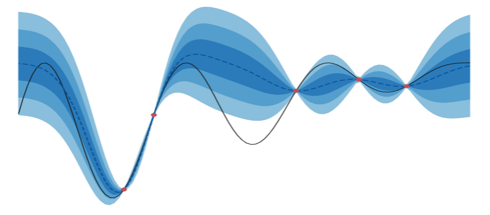
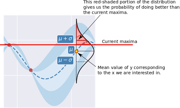
Probability of Improvement (PI) is a good place to start because its intuitive. As the name suggests, at a location \(x\), this calculates the probability of the corresponding \(y\) being greater than the current maxima \(y^*\). Since we’ve a Gaussian distribution of possible output values at \(x\), thanks to the GP, this is calculable in closed form. The image below shows the area under the distribution we’re interested in.

Mathematically, this is what we want to compute at a given \(x\):

In a GP, since \(f(x) \sim \mathcal{N}(\mu(x), \sigma^2(x))\), this can be expressed this in closed form. We will use a change of variables, where \(z=\frac{f(x)-\mu(x)}{\sigma(x)}\) and \(z \sim \mathcal{N}(0,1)\).

This is very convenient since \(\mu(x)\) and \(\sigma(x)\) come from the GP, and \(f(x^*)\) is the current maxima. \(\Phi\) is easily available, e.g., as the cdf function in scipy.

Why Standard Normal?

Something you might wonder about is why did we bother converting to the standard Normal. After all, most languages, including Python/scipy, allow you to create arbitrary Normals, and coding that should have been more convenient.

While that’s correct, there is a practical difference in terms of speed and numerical stability. I’ll address the former first.

Remember you have to find \(argmax_{x \in \mathcal{X}} \alpha_{PI}(x)\), i.e., \(\alpha_{PI}(x)\) needs to evaluated for a lot of \(x\) values. If you instantiate a Normal for each of them, this is going to be slow. Its much faster to use one Normal - the standard Normal here - to process all the data in one shot.

Let me demonstrate. I’ll generate a bunch of random values for means and standard deviations - which we will assume correspond to different \(x\) locations - and I’ll time \(\alpha_{PI}(x)\) in both ways.

import numpy as np
from scipy.stats import norm
import timeit

N = 5000
current_max = 0.7
means = np.random.random(N)
stdevs = np.random.random(N)

different_normals = """\
for m, s in zip(means, stdevs):
    1- norm.cdf(current_max, m, s)
"""

standard_normal = """\
norm.cdf((means-current_max)/stdevs, 0, 1)
"""
repeat = 10
t1 = timeit.timeit(different_normals, globals=globals(), number=repeat)
t2 = timeit.timeit(standard_normal, globals=globals(), number=repeat)

print(f"Using different Normals: {t1/repeat:.04f}")
print(f"Using Standard Normal: {t2/repeat:.04f}")

Here’s the output:

Using different Normals: 0.5551
Using Standard Normal: 0.0004

Using the standard Normal is almost 1400x faster! You can verify the computed values are identical - this is not shown above.

The other reason is numerical stability: working with the standard Normal, and then adjusting the output post-hoc (using something like the Cholesky decomposition), might be less error-prone. We had encountered this idea in the previous post in the context of the GP code.

Expected Improvement

A drawback of PI is that it only looks at the probability of improving and ignores the magnitude of this potential improvement. Expected Improvement (EI) takes that into account by calculating the expected value of the improvement:

Note that values lower than the current maxima are thresholded to \(0\).

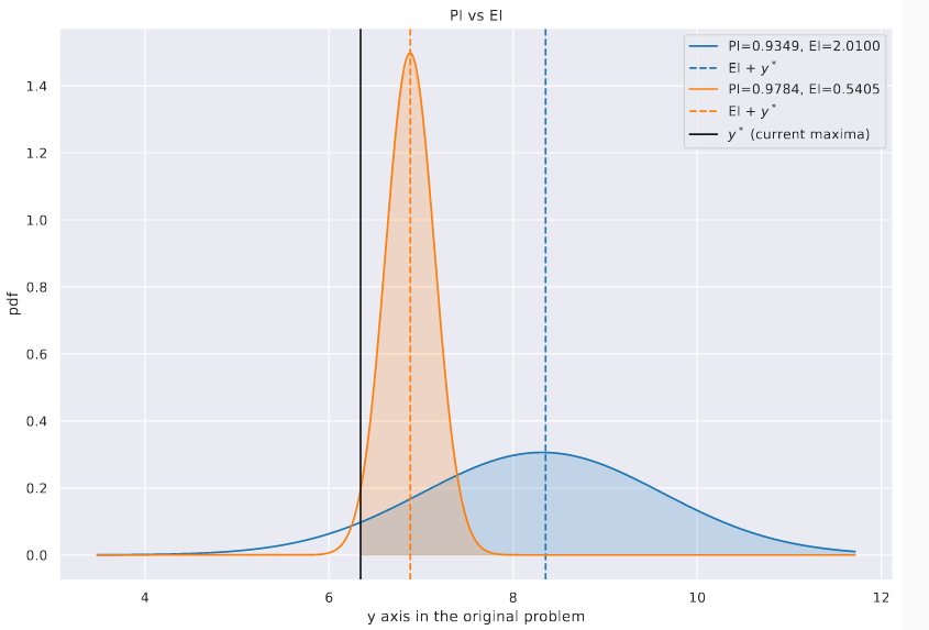
The difference between EI and PI arises in situations where we have a high chance of incremental improvement (favoured by \(\alpha_{PI}\)) vs a relatively low chance of high improvement (favoured by \(\alpha_{EI}\)). In the plot below we show two Gaussians - imagine them as occurring at different values of \(x\) - with the current max shown with a vertical black solid line. The EI and PI values for each are shown in the legend. As you might expect, when asked to pick between them, PI picks the more peaked one (\(\alpha_{PI}=\)0.9784) over the flatter distribution (\(\alpha_{PI}=\)0.9349), while EI picks the latter (\(\alpha_{EI}=\)0.5405 vs \(\alpha_{EI}=\)2.01). Because of this EI may be seen to be more exploratory. EI is also probably the most popular acquisition function for BayesOpt.

EI can be reduced to a closed form expression too. We’ll again use a change of variables: \(z=\frac{f(x)-\mu(x)}{\sigma(x)}\) and \(z \sim \mathcal{N}(0,1)\). In the transformed space, we’ll specifically use \(z^*\) as a shorthand for \(\frac{f(x^*)-\mu(x)}{\sigma(x)}\).

Let’s begin by changing the variables in our expectation. Note that the variable limits are the same, i.e., \(f(x) \to -\infty \implies z \to -\infty\), and \(f(x) \to \infty \implies z \to \infty\).

Thus:

Note above that we now can use the standard Normal’s density \({\color{WildStrawberry}{\varphi(z)}}\). We get rid of the \(max\) by splitting the integral into explicit ranges partitioned at \(z^*\):

Consider the first term:

This colored part is related to \(\varphi(z)\) in the following way:

Hence we can simplify the first term in this manner:

Now, consider the second term:

We’ll use the property that the normal is symmetric about its mean:

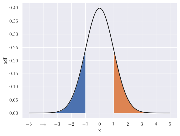
The areas to left of -1 and the right of 1 - shown shaded - are identical.

This allows us to rewrite the limits:

Thus the second term may be simplified as:

Substituting these into the original formula, we have:

Again, we have a concise closed-form expression that maybe computed using the GP (note that \(z^*\) needs \(\mu(x)\) too) and the standard Normal.

Predictive Entropy Search

I won’t go deep into this and the next acquisition functions, and will only try to provide an intuition.

First, some new notation: let \(\hat{x}^*\) and \(\hat{y}^*\) represent the true global maximizer and maximum respectively. This is different from \(x^*\) and \(y^*\), which represent the maxima and maximizer that’s been discovered so far.

One way to assign value to an \(x \in \mathcal{X}\) is in terms of the information gain it provides about the location of the true maximizer \(x^*\). This is Entropy Search (ES) (Hennig & Schuler, 2012):

Here:

• \(\mathcal{D}\) are the function evaluations we have so far.
• \(H[p(t)]\) denotes the entropy of the distribution \(p(t)\). This can be interpreted as the “uncertainty” in the value of \(t\). Roughly, flatter a distribution is, higher is its entropy value. We won’t require its formula per se, but it is calculated as \(H[p(t)]=-\int \!p(t)log \, p(t) \, dt=\mathbb{E}_p[-log \, p(t)]\).
• The first term represents the uncertainty around \(\hat{x}^*\) given observations so far \(\mathcal{D}\). Note that \(x\) - the location for which we’re calculating \(\alpha_{ES}(x)\) - doesn’t show up in this term.
• The second term is similar, but this time we’re interested in the uncertainty if we had observed the function’s value at \(x\), hence the conditioning on \(\mathcal{D} \cup \color{WildStrawberry}{\{x,y\}}\). But we don’t know the exact value for \(y\) - we just have a distribution from the GP - so we calculate the expected uncertainty, which is what \(E_{p\color{WildStrawberry}{(y \vert \mathcal{D}})}\) denotes.
• Putting it all together, the acquisition value for an \(x\) is the amount of reduction in uncertainty about the maximizer it is expected to provide. Greater this reduction, more valuable \(x\) is.

You may have encountered a discrete version of this principle of reduction in entropy before, in Decision Trees such as CART, where it goes by the moniker of Information Gain and is used to determine node splits.

Let’s visualize what we’re after. In the plot below, I have sampled some functions, and visualized their respective maximizers with x. I also have fit a KDE plot - sample max dist. - on the maximizers to show their distribution.

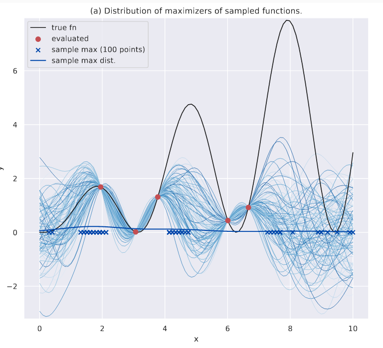
Distribution of maximizers shown.

If I am given more evaluated data, their distribution would obviously change. More sampled functions will begin to agree on the location of the true global maximizer. This is shown in the plot below, where I now have two more evaluations - marked with boxes. Again, note the sample max dist. curve.

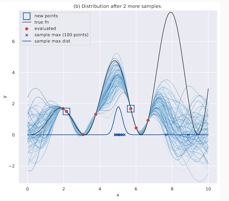
Distribution of maximizers after more evaluations. The maximizers are NOT near the global optima yet, but they seem to agree on a good local maxima.

Effectively, the discrepancy between sampled maximizers has decreased, and this is indicated by the “peakiness” of the KDE plot (the global maxima is still undiscovered, which is a different matter, and further evaluations will redress that). ES uses this as its guiding philosophy: the \(x\) with the greatest acquisition value is the one that leads to the largest decrease in uncertainty of the maximizer’s location.

Direct evaluation of the ES expression is hindered by a few challenges. Let’s look at the expression again:

Here,

• First term: there is no analytic form for \({\color{WildStrawberry}{H[p(\hat{x}^* \vert \mathcal{D})]}}\), and is computable via approximations only.
• Second term: even if we figure out a good way to calculate \(p(\hat{x}^*\vert .)\), it needs to be recomputed for every \(x\) the auxilliary optimizer visits in one BayesOpt iteration since the term \(p(\hat{x}^*\vert \mathcal{D} \cup \{ {\color{WildStrawberry}{x,y}}\})\) is conditioned on \(x\).

Predictive Entropy Search (PES) (Henrández-Lobato et al., 2014) provides an alternate way. The above expression maybe seen as the Mutual Information \(I\) between a point to be acquired and the maximizer (here’s their relationship). And since \(I\) is symmetric, we may rewrite it thus:

Modifying the original equation, we have:

Since \(y\) follows a Gaussian distribution (owing to the GP), \(H[p({\color{WildStrawberry}{y}} \vert x,\mathcal{D})]\) is easy to compute. In the second term, the expectation is wrt \(\color{WildStrawberry}{p(\hat{x}^* \vert \mathcal{D})}\) which doesn’t depend on \(x\), and the target of the expectation, although conditioned on \(x\), doesn’t need \(p(\hat{x}^* \vert .)\) - so we need to approximate \(p(\hat{x}^* \vert \mathcal{D})\) it just once per BayesOpt iteration.

Max-value Entropy Search

Even with the reframing, \(\alpha_{PES}\) might be expensive to compute because of the dependence on \(p(\hat{x}^*)\) when \(\mathcal{X}\) is high-dimensional. But if we were to directly model the maximum, i.e., \(\hat{y}^*\), instead of the maximizer \(\hat{x}^*\), we only have an univariate distribution to deal with. This is exactly what Max-value Entropy Search (MES) (Wang & Jegelka, 2017) does (also see related work in (Hoffman & Ghahramani, 2016)):

The first term is the same as in \(\alpha_{PES}\). However, in the second term, the expectation is wrt \(p(\hat{y}^*\vert \mathcal{D})\), which is univariate, and thus computationally cheaper to compute than \(p(\hat{x}^* \vert \mathcal{D})\).

Additionally, \(\color{WildStrawberry} p(\hat{y}^*\vert\mathcal{D})\) can be approximated by the Gumbel distribution, which describes the maxima of i.i.d. Gaussians (an assumption that’s not true here but works well in practice).

Intuitively, this works a lot like \(\alpha_{PES}\) except we’re looking at the current distribution of \(\hat{y}^*\). As before, the image below shows this distribution for a given \(\mathcal{D}\) - this time the KDE plot is shown on the y-axis.

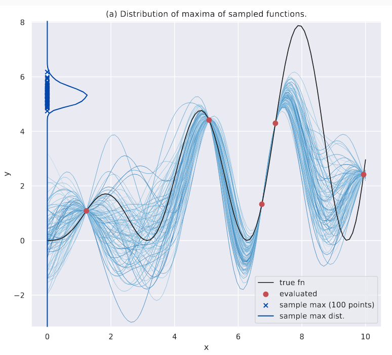
Distribution of the maximum.

As we obtain more evaluations, this distribution becomes peaked. This is what \(\alpha_{MES}\) uses as its guiding principle.

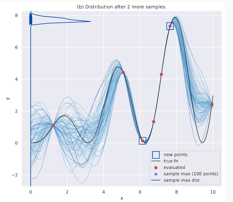
Distribution of the maximum after a few more evaluations.

Something interesting about \(p(\hat{y}^*\vert.)\) is that the density doesn’t go below the current known maximum \(y^*\); because all sampled functions contain this point (remember, function evaluations act as “constrictions”, i.e., all sampled function pass through them, at least in the noiseless GP setting) and therefore their maximum is at least \(y^*\). You can notice these in the above plots as well.

This wraps up our coverage of acquisition functions. Hopefully, we now have a better appreciation of the role of GPs in BayesOpt, in addition to, of course, what the internals of BayesOpt algorithms look like.

Minimal Code for BayesOpt

Are we ready for our own minimal Bayesopt code? You bet!

In the code below, you’ll see an implementation of \(\alpha_{EI}\) in EI(). Our auxiliary optimizer simply samples uniformly in the input space, evaluates \(\alpha_{EI}\) at these points and returns the maximizer. This is not a good optimizer (if we can call it that) compared to say, scipy’s COBYLA, and replacing this with something better would be a good exercise (I feel like some of my teachers who would leave the hardest problems for homework!). But it does the job. Please remember, this is illustrative only, and not meant for serious use! If it helps, imagine this comes with the CRAPL license!

import numpy as np
from sklearn.metrics.pairwise import rbf_kernel as rbf
from scipy.stats import multivariate_normal as mvn, norm


def maximize_by_bayesopt(f, x_min, x_max, iter_budget=100, aux_sample_size=50):

    # create the history arrays
    X_history, y_history = np.zeros(iter_budget), np.zeros(iter_budget)
    # seed with some randomly chosen points - but this is not strictly needed.
    num_random_starts = 5
    X_history[:num_random_starts] = np.random.uniform(x_min, x_max,
                                                      num_random_starts)
    y_history[:num_random_starts] = f(X_history[:num_random_starts])
    current_best = np.max(y_history[:num_random_starts])

    print(f"Finished with {num_random_starts} random calls.")

    # iterate through the remaining iteration budget
    for i in range(num_random_starts, iter_budget):
        print(f"At #iter={i+1} of {iter_budget}.")
        x_next = aux_optimize(current_best=current_best, x_min=x_min,
                              x_max=x_max, X_history=X_history[:i],
                              y_history=y_history[:i],
                              sample_size=aux_sample_size)

        y = f(np.array([x_next]))[0]
        X_history[i], y_history[i] = x_next, y
        print(f"Best so far: {np.max(y_history)}")

    idx_best = np.argmax(y_history)
    x_best, y_best = X_history[idx_best], y_history[idx_best]

    # return the histories to for inspection
    return x_best, y_best, X_history, y_history


def EI(means, stdevs, current_best):
    # the expected improvement acquisition function
    z_stars = (current_best - means)/stdevs
    acq_vals = stdevs * (norm.pdf(z_stars) - z_stars * norm.cdf(-z_stars))
    return acq_vals


def aux_optimize(current_best, x_min, x_max, X_history, y_history,
                 sample_size=50):

    # sample a bunch of points, and return the best
    # this is a very basic "optimizer"
    X_sample = np.random.uniform(x_min, x_max, sample_size)

    # note that we need to reshape to 2D arrays
    mean, cov = gp_predict(X_train=X_history.reshape(-1, 1), y_train=y_history,
                           X_test=X_sample.reshape(-1, 1))
    variances = np.copy(np.diagonal(cov))

    # due to numerical stability issues (of which there are many, when
    # working with matrices!), variances might turn out be very small -ve
    # numbers - we will "fix" it by setting them to a small +ve number.
    # Or you can let them be, and let numpy handle them.
    min_v = np.min(variances)
    if min_v < 0:
        variances[variances < 0] += -min_v + 1e-6
    acq_vals = EI(mean, np.sqrt(variances), current_best)

    return X_sample[np.argmax(acq_vals)]


def gp_predict(X_train, y_train, X_test):
    # this is a pared down version of the earlier gp_predict we saw
    # we don't need sampled functions this time

    # calculate the various partitions
    K_x_x = rbf(X_train, X_train)
    K_x_x_star = rbf(X_train, X_test)
    K_x_star_x = K_x_x_star.T
    K_x_star_x_star = rbf(X_test, X_test)

    # calculate the mean and cov. for the joint output distribution
    mean = K_x_star_x @ np.linalg.inv(K_x_x) @ y_train.reshape((-1, 1))
    mean = mean.flatten()
    cov = K_x_star_x_star - K_x_star_x @ np.linalg.inv(K_x_x) @ K_x_x_star

    return mean, cov

If I wanted to make this code “production ready”, I would at least modify the following aspects:

• Compute the kernel incrementally - note that we’re adding only point per iteration to \(K_{XX}\).
• Deal with numerical stability issues. This is very common when matrix operations are involved. You see that above in how variances has been modified, but the right way to do this would be to fix the cov matrix in gp_predict() first, which leads to faulty variances.
• And of course, we would need a much better auxiliary optimizer.

Anyway, let’s throw a challenge to our bare-bones code: we’ll try maximizing the 1D version of the Ackley function:

# Please ensure that this is in the namespace as the other
# stuff in this section! In other words, copy-paste this in the same
# file or notebook!

def ackley_1D(x):
    a, b, c = 20, 0.2, 6.2
    res = -a * np.exp(-b * x) - np.exp(np.cos(c*x)) + a + 2.7
    return res

Finally, this is how we might visualize BayesOpt’s trajectory:

# Please ensure that this is in the namespace as the other
# stuff in this section! In other words, copy-paste this in the same
# file or notebook!

import matplotlib.pyplot as plt
import seaborn as sns; sns.set()

x_min, x_max = 2, 10
iter_budget = 50

# play around with this value to see how the quality of the aux. optimizer
# influences the search trajectory.
# higher values lead to better search, but slower execution
aux_sample_size = 100

x_best, y_best, X_history, \
y_history = maximize_by_bayesopt(ackley_1D, x_min=x_min, x_max=x_max,
                                 iter_budget=iter_budget,
                                 aux_sample_size=aux_sample_size)


fig = plt.figure(figsize=(12, 8))
ax = fig.add_subplot(111)

# plot the original fn
X = np.linspace(x_min, x_max, 1000)
sns.lineplot(x=X, y=ackley_1D(X), ax=ax)

# make the scatter sizes correspond to recency, i.e.,
# points recent in the history look bigger
g = sns.scatterplot(x=X_history, y=y_history,
                    size=np.arange(len(X_history))+1,
                    sizes=(50, 200), ax=ax)

# remove the legend since it shows the dot sizes,
# and these are not relevant
g.legend([], [], frameon=False)

# draw a vert. line at the discovered maxima
ax.axvline(x=x_best, linestyle='--', c='r')

# annotate the plot
ax.set_xlabel('x'); ax.set_ylabel('y')
ax.set_title(f"aux. opt.=random sampling, # iter: {iter_budget}, "
             f"aux. sample size={aux_sample_size}")

plt.show()

Points visited by BayesOpt are sized wrt recency - recent points are larger. This is the output of the above code:

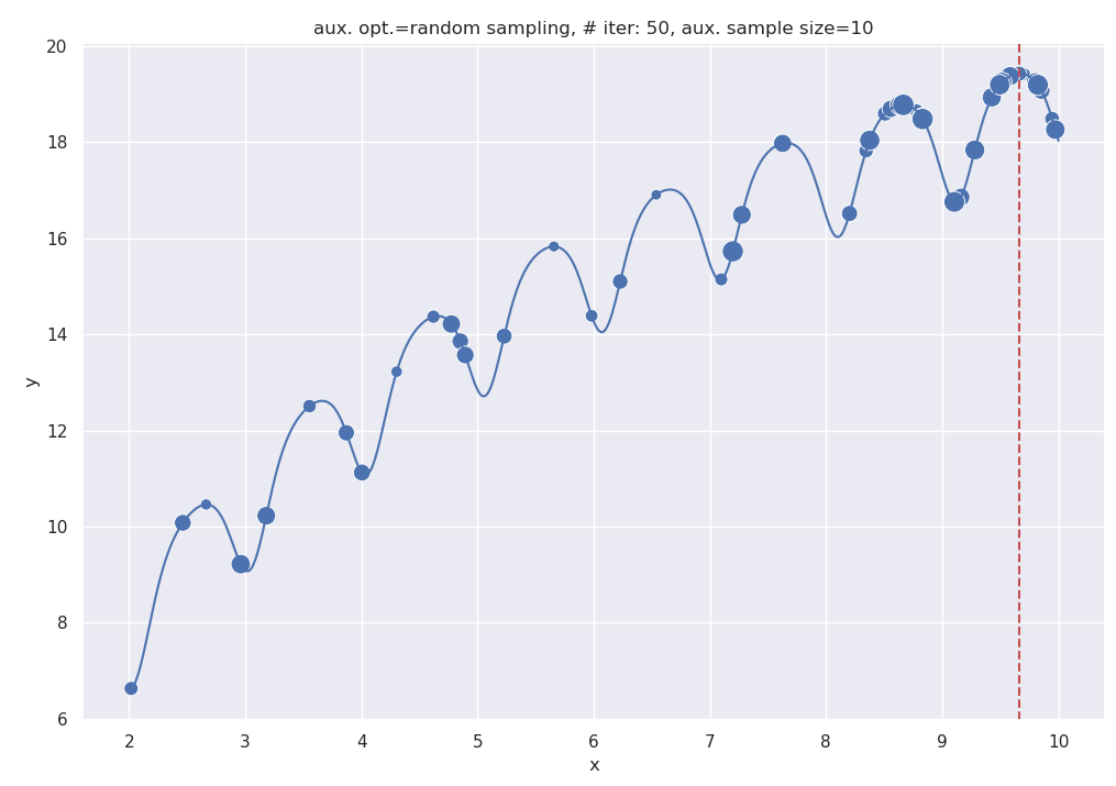
Output of the BayesOpt code, with a sample size of 10 for the aux. optimizer.

One advantage of using the simple auxiliary optimizer here is we can analyze the effect of the quality of this optimizer on the final outcome. For ex., setting aux_sample_size = 100 gives us a better auxiliary optimizer since it explores more of the input space. At even higher numbers, it would discover the acquisition maxima almost by brute-force.

The following plot shows the output for aux_sample_size = 100. If you compare this plot with the previous one, you’ll notice that a lot more points here are concentrated at the rightmost hump, as opposed to the rightmost two in the previous one. This indicates faster convergence to the maxima.

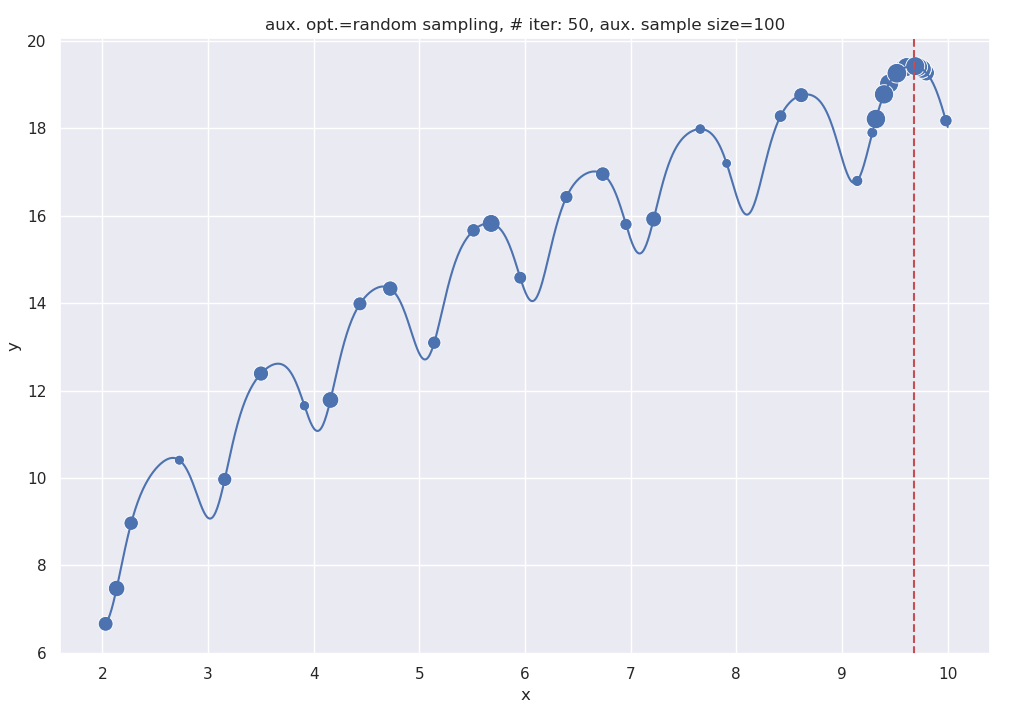
Output of the BayesOpt code, with a sample size of 100 for the aux. optimizer.

Summary, a Pet Peeve and Learning Resources

We’re finally at the end of our (somewhat long) discussion of BayesOpt. One way to think of BayesOpt is as a middleman between a real-world function and black-box optimizers such as CMA-ES (the auxiliary optimizers), that aren’t sample-efficient. BayesOpt coaxes these into working by supplying them with hallucinated functions from the surrogate model. And by observing what they find, e.g., where does the extrema (of these simulated functions) typically lie? How large/small is this extrema?, it estimates the informativeness of various input regions. Accordingly, it requests the real-world function for a specific evaluation. The response is used to adjust the surrogate model, and then the whole process of enlisting the auxiliary optimizers to operate over simulated functions begins anew.

Torturing this metaphor further, you might wonder, “Hey, this seems like a fairly general way to compute other properties of functions, not just optima! Just replace CMA-ES with an arbitrary algorithm!”. And you’d be right - this is exactly the kind of extension InfoBAX (Neiswanger et al., 2021) proposes.

While we looked at the canonical versions of BayesOpt, I’d point out that because of the plug-and-play nature of the framework - you can replace one or more of the following: surrogate model, acquisition function, kernel - BayesOpt is extremely versatile. It has been adapted for combinatorial search in discrete structured spaces (Papenmeier et al., 2023; Baptista & Poloczek, 2018; Deshwal et al., 2020; Deshwal & Doppa, 2021), parallelization (Wang et al., 2020; Kandasamy et al., 2018), sparsity (McIntire et al., 2016; Liu et al., 2023), has been used with Neural Networks as the surrogate model (Snoek et al., 2015; Springenberg et al., 2016), has been paired with other optimizers such as Gradient Descent (Wu et al., 2017) and Hyperband (Falkner et al., 2018), and has gained some new acquisition functions (Ament et al., 2023; Moss et al., 2021; Wilson et al., 2017) along the way. The list of applications is impressively diverse - from hyperparameter optimization to plasma control in nuclear fusion (Mehta et al., 2022) and Molecular Property Optimization (Sorourifar et al., 2023). The preamble to the part 1 post lists some more.

So what’s this about a pet peeve? Well, consider the case of hyperparameter optimization. We know BayesOpt works empirically, but BayesOpt has parameters too (these could be kernel, surrogate model or acquisition function parameters) - why is tuning them not necessary, or to put it optimistically, how do know that the underlying problem is insensitive to BayesOpt’s parameters? What’s stopping me from slapping on another BayesOpt algo on top of the first to tune its parameters, and then another on top of that one, and so on? It seems to me that there is place for theoretical results like the No Free Lunch theorem in this area.

Anyway, notwithstanding that, this is an exciting area!

If you’re picking up BayesOpt, I’d recommend these resources:

• Gaussian Processes - My favorite is this talk by Richard Turner (the first 30 min are an excellent intro to GPs). Nando De Freitas also a great talk on GPs where he has some code examples. The book Bayesian Reasoning and Machine Learning (Barber, 2012) has a chapter dedicated to GPs and covers the topic well. On a tangential note, I think the book is quite underrated, but luckily, available online. As mentioned in the previous post, David Duvenaud has a catalogue of kernels here. Of course, the standard text in the area is Rasmussen and Williams’ Gaussian Processes for Machine Learning (Rasmussen & Williams, 2005), which is available here. I came across Gregory Gundersen’s blog last year, which does a great job of covering some of the mathematical aspects of GPs.
• Bayesian Optimization - Nando De Freitas has a talk on BayesOpt. I also recommend this popular tutorial (Shahriari et al., 2016). I came across this book by Roman Garnett (Garnett, 2023) recently and I found it well-organized and helpful. The book had appeared on Hacker News, where the author had participated in the discussion. Matthew Hoffman’s talk at UAI-2018 is quite good too.

References

1. Hennig, P., & Schuler, C. J. (2012). Entropy Search for Information-Efficient Global Optimization. J. Mach. Learn. Res., 13(null), 1809–1837.
2. Henrández-Lobato, J. M., Hoffman, M. W., & Ghahramani, Z. (2014). Predictive Entropy Search for Efficient Global Optimization of Black-Box Functions. 918–926.
3. Wang, Z., & Jegelka, S. (2017). Max-value Entropy Search for Efficient Bayesian Optimization. In D. Precup & Y. W. Teh (Eds.), Proceedings of the 34th International Conference on Machine Learning (Vol. 70, pp. 3627–3635). PMLR. https://proceedings.mlr.press/v70/wang17e.html
4. Hoffman, M. W., & Ghahramani, Z. (2016). Output-Space Predictive Entropy Search for Flexible Global Optimization.
5. Neiswanger, W., Wang, K. A., & Ermon, S. (2021). Bayesian Algorithm Execution: Estimating Computable Properties of Black-box Functions Using Mutual Information. In M. Meila & T. Zhang (Eds.), Proceedings of the 38th International Conference on Machine Learning (Vol. 139, pp. 8005–8015). PMLR. https://proceedings.mlr.press/v139/neiswanger21a.html
6. Papenmeier, L., Nardi, L., & Poloczek, M. (2023). Bounce: Reliable High-Dimensional Bayesian Optimization for Combinatorial and Mixed Spaces. Thirty-Seventh Conference on Neural Information Processing Systems. https://openreview.net/forum?id=TVD3wNVH9A
7. Baptista, R., & Poloczek, M. (2018). Bayesian Optimization of Combinatorial Structures. In J. Dy & A. Krause (Eds.), Proceedings of the 35th International Conference on Machine Learning (Vol. 80, pp. 462–471). PMLR. https://proceedings.mlr.press/v80/baptista18a.html
8. Deshwal, A., Belakaria, S., & Doppa, J. R. (2020). Scalable Combinatorial Bayesian Optimization with Tractable Statistical models. ArXiv Preprint ArXiv:2008.08177.
9. Deshwal, A., & Doppa, J. (2021). Combining Latent Space and Structured Kernels for Bayesian Optimization over Combinatorial Spaces. In A. Beygelzimer, Y. Dauphin, P. Liang, & J. W. Vaughan (Eds.), Advances in Neural Information Processing Systems. https://openreview.net/forum?id=fxHzZlo4dxe
10. Wang, J., Clark, S. C., Liu, E., & Frazier, P. I. (2020). Parallel Bayesian Global Optimization of Expensive Functions. Operations Research, 68(6), 1850–1865. https://doi.org/10.1287/opre.2019.1966
11. Kandasamy, K., Krishnamurthy, A., Schneider, J., & Poczos, B. (2018). Parallelised Bayesian Optimisation via Thompson Sampling. In A. Storkey & F. Perez-Cruz (Eds.), Proceedings of the Twenty-First International Conference on Artificial Intelligence and Statistics (Vol. 84, pp. 133–142). PMLR. https://proceedings.mlr.press/v84/kandasamy18a.html
12. McIntire, M., Ratner, D., & Ermon, S. (2016). Sparse Gaussian Processes for Bayesian Optimization. Proceedings of the Thirty-Second Conference on Uncertainty in Artificial Intelligence, 517–526.
13. Liu, S., Feng, Q., Eriksson, D., Letham, B., & Bakshy, E. (2023). Sparse Bayesian optimization. In F. Ruiz, J. Dy, & J.-W. van de Meent (Eds.), Proceedings of The 26th International Conference on Artificial Intelligence and Statistics (Vol. 206, pp. 3754–3774). PMLR. https://proceedings.mlr.press/v206/liu23b.html
14. Snoek, J., Rippel, O., Swersky, K., Kiros, R., Satish, N., Sundaram, N., Patwary, M., Prabhat, M., & Adams, R. (2015). Scalable Bayesian Optimization Using Deep Neural Networks. In F. Bach & D. Blei (Eds.), Proceedings of the 32nd International Conference on Machine Learning (Vol. 37, pp. 2171–2180). PMLR. https://proceedings.mlr.press/v37/snoek15.html
15. Springenberg, J. T., Klein, A., Falkner, S., & Hutter, F. (2016). Bayesian Optimization with Robust Bayesian Neural Networks. In D. Lee, M. Sugiyama, U. Luxburg, I. Guyon, & R. Garnett (Eds.), Advances in Neural Information Processing Systems (Vol. 29). Curran Associates, Inc. https://proceedings.neurips.cc/paper_files/paper/2016/file/a96d3afec184766bfeca7a9f989fc7e7-Paper.pdf
16. Wu, J., Poloczek, M., Wilson, A. G., & Frazier, P. (2017). Bayesian Optimization with Gradients. In I. Guyon, U. V. Luxburg, S. Bengio, H. Wallach, R. Fergus, S. Vishwanathan, & R. Garnett (Eds.), Advances in Neural Information Processing Systems (Vol. 30). Curran Associates, Inc. https://proceedings.neurips.cc/paper_files/paper/2017/file/64a08e5f1e6c39faeb90108c430eb120-Paper.pdf
17. Falkner, S., Klein, A., & Hutter, F. (2018). BOHB: Robust and Efficient Hyperparameter Optimization at Scale. In J. Dy & A. Krause (Eds.), Proceedings of the 35th International Conference on Machine Learning (Vol. 80, pp. 1437–1446). PMLR.
18. Ament, S., Daulton, S., Eriksson, D., Balandat, M., & Bakshy, E. (2023). Unexpected Improvements to Expected Improvement for Bayesian Optimization. Thirty-Seventh Conference on Neural Information Processing Systems. https://openreview.net/forum?id=1vyAG6j9PE
19. Moss, H. B., Leslie, D. S., Gonzalez, J., & Rayson, P. (2021). GIBBON: General-purpose Information-Based Bayesian Optimisation. Journal of Machine Learning Research, 22(235), 1–49. http://jmlr.org/papers/v22/21-0120.html
20. Wilson, J. T., Moriconi, R., Hutter, F., & Deisenroth, M. P. (2017). The Reparameterization Trick for Acquisition Functions. NIPS Workshop on Bayesian Optimization. https://bayesopt.github.io/papers/2017/32.pdf
21. Mehta, V., Paria, B., Schneider, J., Neiswanger, W., & Ermon, S. (2022). An Experimental Design Perspective on Model-Based Reinforcement Learning. International Conference on Learning Representations. https://openreview.net/forum?id=0no8Motr-zO
22. Sorourifar, F., Banker, T., & Paulson, J. (2023). Accelerating Black-Box Molecular Property Optimization by Adaptively Learning Sparse Subspaces. NeurIPS 2023 Workshop on Adaptive Experimental Design and Active Learning in the Real World. https://openreview.net/forum?id=JJrwnclCFZ
23. Barber, D. (2012). Bayesian Reasoning and Machine Learning. Cambridge University Press.
24. Rasmussen, C. E., & Williams, C. K. I. (2005). Gaussian Processes for Machine Learning (Adaptive Computation and Machine Learning). The MIT Press.
25. Shahriari, B., Swersky, K., Wang, Z., Adams, R. P., & de Freitas, N. (2016). Taking the Human Out of the Loop: A Review of Bayesian Optimization. Proceedings of the IEEE, 104(1), 148–175. https://doi.org/10.1109/JPROC.2015.2494218
26. Garnett, R. (2023). Bayesian Optimization. Cambridge University Press.