The Gumbel-Max Trick

When we set out to learn a function or some property of it (like its maximum), we hope it is differentiable, because that means we have at our disposal a host of well-studied, and often fast, techniques. But sometimes we are not so lucky - and then there are broadly two options: (a) use a technique that doesn’t rely on differentiability, e.g., Bayesian Optimization, or (b) use an approximation that is differentiable. The topic of this post is a very useful and elegant instance of the latter. It’s a technique to make sampling from a categorical distribution differentiable, using the Gumbel distribution (McFadden, 1974; Jang et al., 2017; Maddison et al., 2017). The need to differentiate through the categorical distribution shows up in various places (Huijben et al., 2023). JAX implements a differentiable version of categorical sampling using the Gumbel-max trick. About it this paper (Kool et al., 2019) says:

We think the Gumbel-Max trick is like a magic trick.

I agree! Let’s get started.

• Why Differentiability
• The Problem with Sampling
• Outline
• The Gumbel-Max Trick
• Softmax Approximation
• Pit Stop
• Toy Problem - Modeling a Biased Die
• References

Why Differentiability

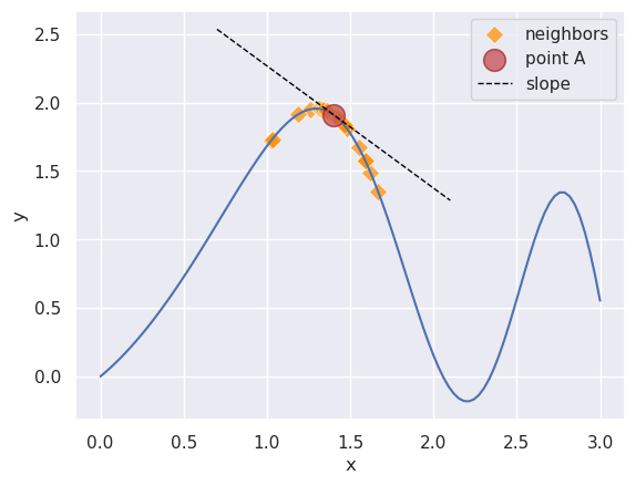
Let’s quickly understand why differentiability is a big deal. Let’s say we are minimizing a function. And right now, we know the value of the function at the location of point A.

Two situations arise:

• If the function is differentiable, we have the gradient at A, i.e., \(\frac{dy}{dx}\) - represented with the black dashed line. This line tells us what the vicinity of A looks like:
  • It tells us which direction trends down (right) vs up (left). Since we are interested in the minima, we can choose to move to the right of A.
  • Moreover, the gradient’s magnitude tells us how much we want to move in that direction, e.g., if it is low, we might be near the minima and we should move slowly so as to not overstep it.
• If it is not differentiable, we will have to guess the structure of the landscape around A. For example, we might do this by evaluating the function repeatedly in A’s neighborhood. This is shown with the diamond markers.

Differentiability gives us valuable information about where and how much to move. Gradient Descent techniques, such as ADAM and Muon, utilize this information and focus our search for the minima on the most promising regions of the function. The value of the gradient information is efficiency: it lets us avoid massive swathes of the function landscape. Lacking differentiability, we have to explicitly gather this information, e.g., approximation via neighbors, making search expensive.

When we set up a neural network, say in PyTorch, we’re indirectly constructing a function that is differentiable: every building block, e.g., nodes or layers with specific operations, that we use is differentiable (ReLU needs special handling), which makes their assembly - the entire network - differentiable. Stitching the individual pieces together may be thought of as function composition operations; thus, calculating the derivative is essentially an application of the chain rule.

The Problem with Sampling

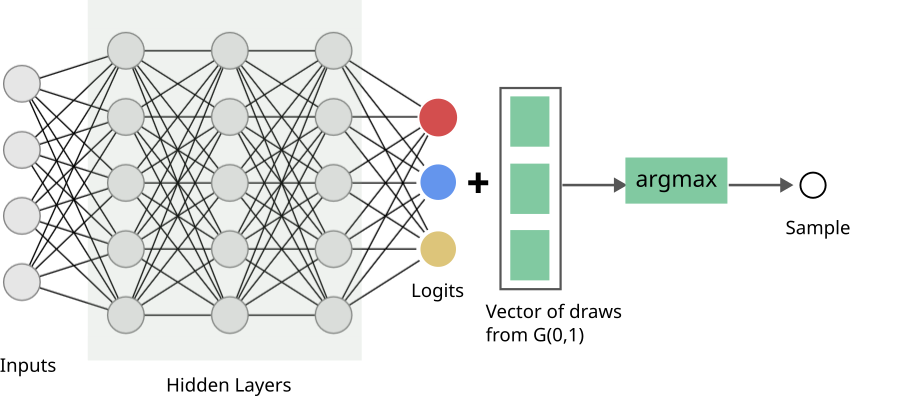
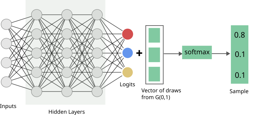
Consider a scenario where we are learning a network that produces parameters of a categorical distribution; this distribution describes \(K\) possible events that can occur with respective probabilities \(p_0, p_1, ..., p_{K-1}\), and is often written as \(Cat(p_0, p_1, ..., p_{K-1})\). There are scenarios where the loss is defined on a sample you draw from the distribution. The below schematic shows what this might look like: a “standard” neural network till we get to the parameters of the distribution (often called logits - while these are real numbers \(\in (-\infty, \infty)\), these can be transformed into distribution parameters easily - I’ll clarify later in the post), and then there is a sampling step.

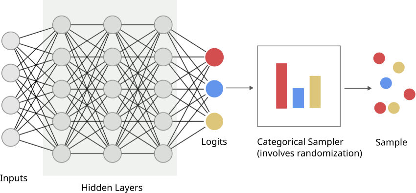
Now, when you’re generating a sample, you’re relying on some form of randomness; typically a random number generator that your programming language uses. There is no gradient here, i.e., the gradient flows from the logits backwards just fine, but there is no way to go from the loss to the logits via the sampling step.

Let me put this another way: the loss depends on the sample, which depends on the distribution’s parameters, which depends on the current weights of the network. Intuitively, to reduce the loss, we should nudge the distribution parameters, and thus the network weights, towards a favorable direction. But there is no direct mechanism to connect the sample loss to a nudge to the distribution parameters via a gradient, and therefore, gradient-based techniques are seemingly off the table.

The Gumbel-Max trick provides a workaround.

Outline

There are really two parts to the trick, and I’m splitting their description across the following two sections. At a high-level, this is what ends up happening:

• We separate out the randomness in sampling in a way that it does not depend on network parameters. Which means you can ignore the randomizing step when calculating the gradient - just as you’d ignore a term that does not depend on the thing we’re differentiating with, e.g., a constant. Technically, this is the Gumbel-max trick.
• The above fix leads to a new differentiability problem - this time of finding the gradient of the “maximum” operation, i.e., find the maximum of a set of numbers. Fortunately, we’re able to use a well-known solution to this, using the softmax operation. This bit is commonly referred to as the Gumbel-softmax relaxation.

It took me a while to decide if I should call the post the “Gumbel-Max Trick” or the “Gumbel-Softmax Trick”. I decided to go with the former because I find the relevant math very interesting.

The Gumbel-Max Trick

For a while, let’s forget the neural network, and only talk distributions.

The Gumbel distribution is a type of extreme value distribution. The latter is what you get when you take multiple samples from a distribution and look at the distribution of only the sample maximums (or minimums). Below, I have taken three distributions - a Normal, an Exponential, and a mixture of two Normals, shown by the line curves. In each case, I sampled (sample size=100) from these distributions 1000 times and drew a filled KDE plot fitted to the 1000 sample maxima.

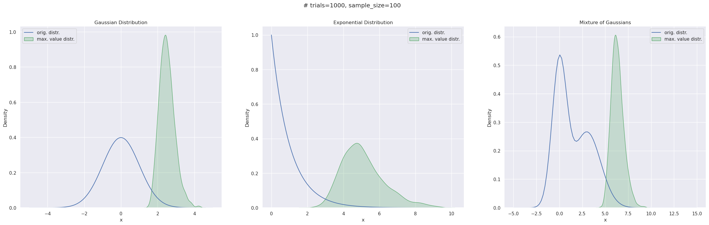
One thing to note here is these empirical distributions have a right skew, i.e., a right tail - which is probably not surprising given they’re constituted solely by sample maximums.

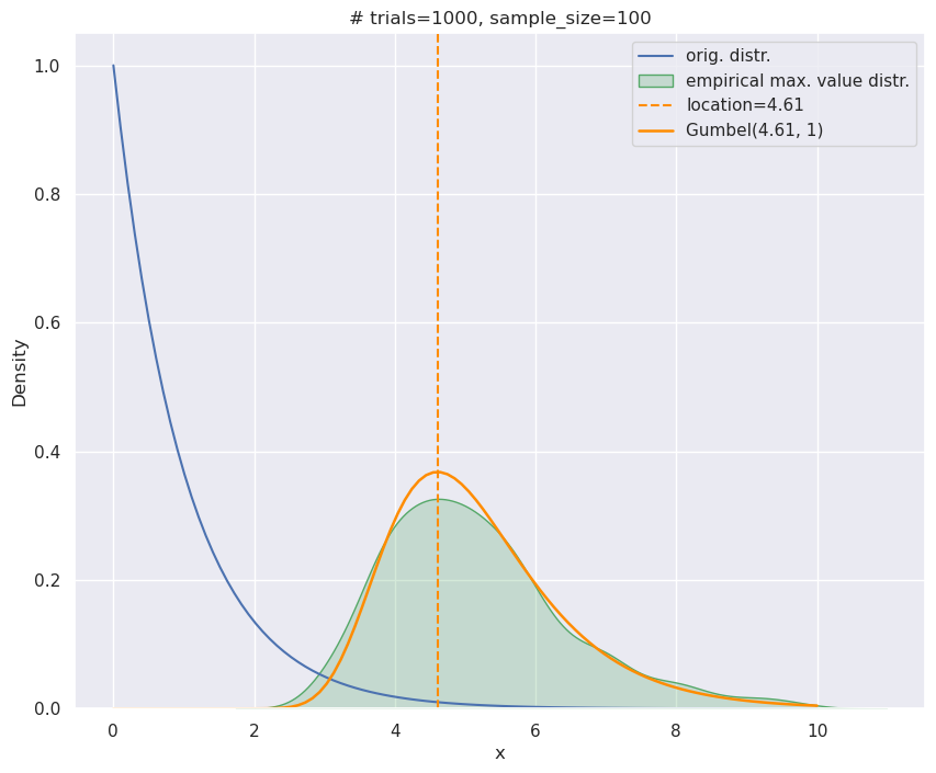
For the Exponential distribution (the middle plot) it is possible to define this distribution analytically. And that’s the Gumbel distribution. Its probability density function (\(\texttt{pdf}\)) is written as \(G(\mu, \beta)\):

\(\mu\) and \(\beta\) are known as location and scale respectively. In this post, we’ll only need to use \(\beta=1\), so I’ll entirely drop the symbol. scipy has an implementation if you want to try it out. Below I have redrawn the empirical maximum value distribution for the Exponential - like in the middle plot above - and have also shown the corresponding Gumbel distribution (with appropriate shifting/scaling). They match pretty well, and of course, one sees the right skew here too.

The Gumbel distribution has two properties of interest to us. Things are going to get a little mathy, and if you want to skip the proofs, just note the claims themselves - marked with 🔺- because those will get used later in the section.

• Property 1: 🔺Sampling from \(G(a, 1)\) is equivalent to sampling from \(G(0,1)\) and adding \(a\) to the sampled values.

  Proof: We reinterpret the statement above: if I sample a bunch of \(x\)s from \(G(0,1)\), and add \(a\) to them, they’re as good as samples from \(G(a,1)\). In other words: the \(\texttt{pdf}\) value of \(x \sim G(0, 1)\) and \((x+a) \sim G(a,1)\) are identical. Let’s consider \(p(x+a\vert G(a,1))\). This is the \(z\) we’ll have to use in the \(\texttt{pdf}\) expression (see Gumbel \(\texttt{pdf}\) above):

  \[z = ((x+a)-a) = x\]

  But \(z=x\) is also what we need to use in the \(\texttt{pdf}\) for \(G(0, 1)\). Hence the probability of sampling \(x \sim G(0,1)\) and \(x+a \sim G(a,1)\) are identical.

• Property 2: 🔺Sampling from the categorical distribution, i.e., \(x \sim Cat(p_0, p_1, ..., p_{K-1})\) is equivalent to independently sampling a value each from \(K\) separate Gumbels \(G(log\;p_0, 1)\), \(G(log\;p_1, 1)\), …, \(G(log\;p_{K-1}, 1)\) and finding out which distribution produced the maximum.

  I’ll be using this new notation here: \(I\) will be a shorthand for the set \(\{0,1, .., K-1\}\). To denote that I want element \(i\) removed from the set, I’ll write \(I/i\).

  🔺Let’s formalize our claim - we are saying that for \(x_i \sim G(log\;p_i, 1)\) and a specific category \(k\):

  \[p(x_k > x_j) = p_k,\;\text{where } j \in I/k\]

  Note that \(p_k\), our RHS, is the probability of category \(k\) being picked when sampling from the categorical distribution.

  Before we get to a proof, I’d point out that part of this is intuitive. Since \(log\) is monotonic, a greater \(p_i\) means that its corresponding Gumbel, located at \(log\;p_i\), would be shifted farther to the right side of the x-axis, compared to a lower \(p_i\). Plus there is the right skew of the Gumbel which would emphasize this ordering. So, a higher \(p_i\) implies that both category \(i\) is likely to be picked from the categorical distribution, and the value from the Gumbel is likely to be the largest.

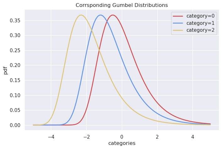
  For ex., here’s a categorical distribution with \(K=3\):

  

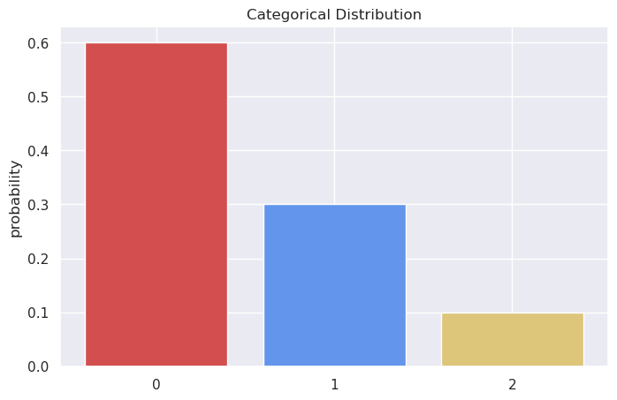
  And here are the corresponding Gumbels - clearly, if we sample from them independently and find the maximum, we’ll end up with category 0 as the winner relatively more often.

  

  The surprising bit is their exact equivalence!

  Proof: I’m going to use some Gumbel properties to make the proof concise - it shouldn’t be too hard to find proofs from scratch online.

  So, first off, let’s ask if \(x_a \sim G(a, 1)\) and \(x_b \sim G(b, 1)\), what might be the probability of \(p(x_a>x_b)\)?

  Gumbels have this interesting property that \(x_a-x_b\) follows a Logistic Distribution whose cumulative distribution function (cdf) is \(F_X(x)=1/(1+e^{-(x-(a-b))})\). Here \(X\) is a random variable that follows the Logistic Distribution. Recall that \(F_X(x)\), i.e., the \(\text{cdf}\), represents \(p(X \leq x)\).

  Since we want \(p(X>0)\), where \(X=x_a-x_b\), all we need is to calculate \(1 - p(X \leq 0 )\) or \(1-F(0)\). This is:

  \[1 - \frac{1}{1+e^{a-b}} = \frac{e^{a-b}}{1+e^{a-b}}\]

  Looks complicated. But let’s say that \(a=log\; p_a\) and \(b=log\; p_b\). This simplifies things quite a bit, and we have:

  \[\frac{e^{log\; \frac{p_a}{p_b}}}{1 + e^{log\;\frac{p_a}{p_b}}} = \frac{p_a}{p_a+p_b}\]

  This is intuitive: larger \(p_a\) is (relatively), its Gumbel shifts farther to the right on the x-axis, leading to greater possibility of \(x_a > x_b\).

  OK, so we have inferred an interesting relationship. How does that help us? Remember, what we really want to show is \(p(x_k > x_j) = p_k, \forall j \in I/k\). We can rephrase that to find:

  \[p(x_k > max_{j \in I/k}\{x_j\} )\]

  Effectively, we’re saying that \(x_k > x_j\) is the same as \(x_k\) being larger than the maximum of the rest of the Gumbel samples. Another property is helpful here: the maximum of independent Gumbels with the same scale (true for us - all scales are \(1\)) is also a Gumbel! This property allows us to rewrite the RHS:

  \[max_{j \in I/k}\{x_j\} = G(log\; \sum_{j \in I/k} e^{log\;p_j}, 1 )\]

  This simplifies to \(G(log\; \sum_j p_j, 1)\). So now we’re asking what’s the probability that a sample from \(G(log\;p_k, 1)\) is larger than one from \(G(log\; \sum_j e^{log\;p_j}, 1 )\). But hey, we just found the answer to this! This probability is:

  \[\frac{p_k}{p_k + \sum_{j \in I/k} p_j} = p_k\]

  The denominator is the sum of the all the categorical probabilities and therefore must sum to \(1\). So the probability we set out to find is just \(p_k\).

How do these properties help us with the big picture? Combining the two properties above, the new recipe for sampling from \(Cat(p_0, p_1, ..., p_{K-1})\) is:

• For category \(0\), sample from \(G(log\;p_0, 1)\). Or by Property 1, sample from \(G(0,1)\) and add \(log\;p_0\) to the sample.
• For category \(1\), add \(log\;p_1\) to a sample from \(G(0,1)\).
• For category \(2\), add \(log\;p_2\) to a sample from \(G(0,1)\).
• … so on …
• Find which category produced the maximum value.

Referring to the \(i^{th}\) sample from \(G(0,1)\) as \(g_i\), we may distill this recipe as follows:

To connect this back to our neural network pipeline, we’ll need to circle back to the logits - the values we actually get from the last layer. Let’s refer to these as \(l_i\) and assume we’ve \(K\) of these. Note that \(l_i \in (-\infty, \infty)\). These may be transformed into probabilities, i.e., for every \(l_i\) we can create a \(p_i\) such that \(0 \leq p_i \leq 1\) and \(\sum_{i \in I}p_i = 1\) in the following way:

The denominator doesn’t depend on \(i\), so we’ll represent it with the constant \(C=\sum_{j \in I} e^{l_j}\). Then we have \(log\;p_i=l_i-log\;C\). It follows that:

This is because subtracting the same constant term from each of the quantities we’re \(argmax\)-ing over doesn’t change where the maximum occurs, i.e., the \(argmax\). It reduces the maxima itself - by \(log\;C\) - but we’re not interested in it. So now we have connected our new sampling strategy to the outputs of the network: add each logit \(l_i\) to a sample from \(G(0,1)\) and report the \(i\) where the sum is the largest.

Look at the strategy closely - we have managed to decouple the network parameters/outputs from the randomness! This is a form of reparameterization. The randomness is produced by \(G(0,1)\) which doesn’t depend on any network or distribution parameter. Which means when we calculate derivatives we can safely ignore the sampling step, in the same way you ignore constant terms. This is the magic part of the trick: categorical \(\to\) Gumbel \(\to\) just the standard Gumbel.

This is what our network looks like now:

We have a new hiccup though: \(argmax\) is also not differentiable. And this we can’t ignore - because it operates over a quantities that use the network’s outputs, i.e., the logits. Thankfully, this is an easier problem to solve.

Softmax Approximation

If you haven’t already guessed, the solution is to replace the \(argmax\) with the standard \(softmax\). This gives us a \(K\)-dimensional vector. For index \(i\), we now compute:

\(\tau\), the temperature, decides the discreteness of the \(softmax\); ideally we want only one dimension in this vector have a value of \(1\) while everything else is set to \(0\), to perfectly mimic \(argmax\). But this is not differentiable. \(\tau\) makes the vector smooth, i.e., spreads values across dimensions. Larger \(\tau\) values promote this spread, making gradient-based optimization easier, while lower values better mimic \(argmax\). The standard process is to anneal the value for \(\tau\), i.e., start with a high value, but gradually lower it over iterations. Here’s how \(\tau\) affects the final values - note, how at at \(\tau=0.1\) this behaves like \(argmax\):

This \(softmax\)-ed vector is our (one) sample. The distribution of samples thus obtained is known as the Gumbel-Softmax distribution (Jang et al., 2017). Here’s our final network:

Now, ignoring the vector from the standard Gumbel, which we have painstakingly proved we’re allowed to do, everything is differentiable!

Pit Stop

Before we move on, let me quickly summarize what we’ve found:

• We started with the problem of not being able to find gradients when a network’s loss depended on a sampling step. Specifically because there was random number generation involved.
• We came up with a reparameterization, that usefully decomposed the problem: we got a part that depends on the network parameters (the logits) and a part that was independent of the network, which actually does the sampling. Note: we could have done performed sampling earlier too - there is nothing difficult about sampling directly from a categorical distribution. But the value of the decoupling is in allowing the gradient to ignore the sampling step. This is the Gumbel-max trick.
• As luck would have it, our fix led to another non-differentiability: the \(argmax\). But this turned out to be a simpler problem to resolve by replacing the \(argmax\) with \(softmax\). This is the Gumbel-softmax relaxation.

Toy Problem - Modeling a Biased Die

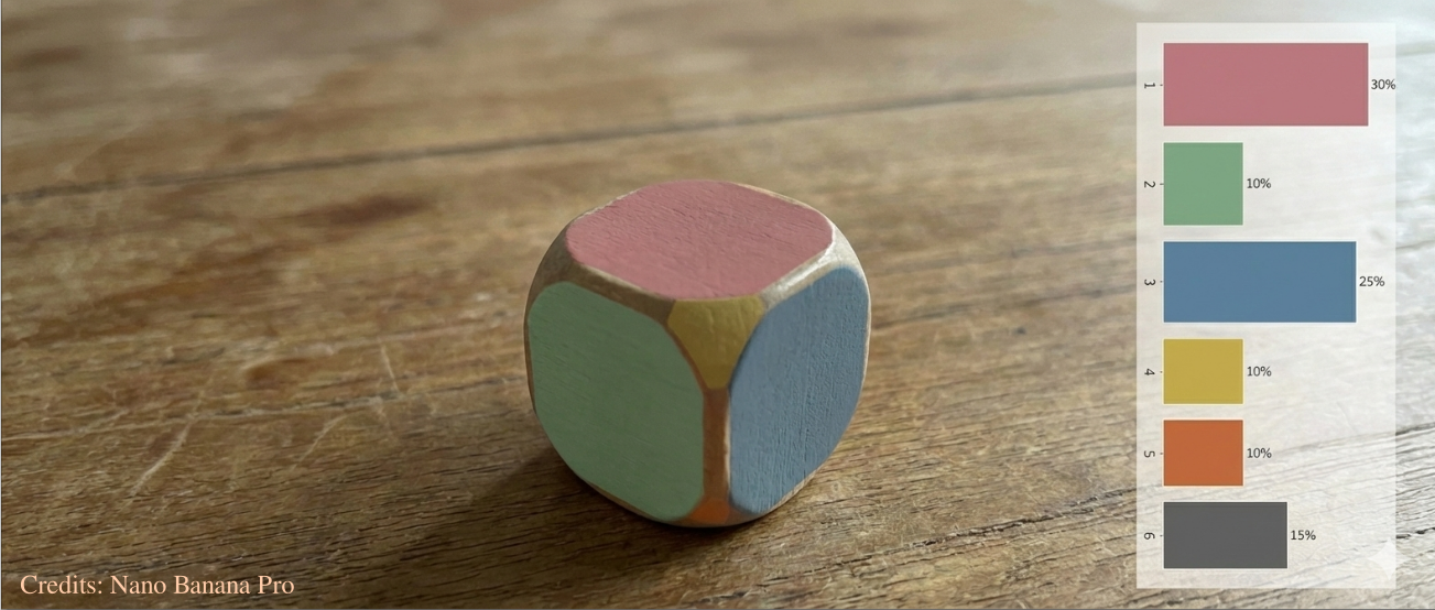
We will look at a toy problem of modelling the categorical distribution for a biased die. This will help us appreciate the mechanics up close. For an example using a Variation Autoencoder (VAE), Eric Jang, one of the authors of the Gumbel-softmax paper (Jang et al., 2017), has an example on his blog.

Here’s the problem we’ll solve: We are going to learn the probabilities of each face coming up for a 6-sided die. We will roll the die a few times, and report the fraction of times each face came up. For example, if we roll it thrice and see:

• 0, 0, 0, 1, 0, 0 - here “\(1\)” at a position indicates the corresponding face shows up on top.
• 1,0, 0, 0, 0, 0
• 1, 0, 0, 0, 0, 0

Then we report the numbers \([0.67, 0, 0, 0.33, 0, 0]\); let’s call this our observation vector.

We use this observation to train our logits \(l_i\) directly. Yes, to keep things simple, we won’t be looking at a full-fledged network. The logit values will be our starting point, which we’ll learn using gradient descent. We’ll compare one softmax sample with the observation vector we created above, using the Sum of Squared Errors (SSE) loss. Let’s say our one softmax sample is \([0.1, 0.1, 0.1, 0.3, 0.2, 0.2]\). The SSE value then is:

\((0.67-0.1)^2 + (0-0.1)^2 + (0-0.1)^2 + (0.33-0.3)^2+ (0-0.2)^2+ (0-0.2)^2=0.4258\).

You can use other losses - KL Divergence is popular - but we want to keep it simple here.

OK, so we get this SSE, and based on this, calculate the gradient. And based on that, we update our logits. All of this is repeated till we’re happy with the results. Let’s begin by focusing on how the logits get transformed:

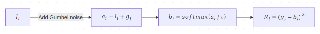
• We start with the logits vector \(l\), where \(l_i\) is the logit for the \(i^{th}\) category.
• We add standard Gumbel noise to obtain vector \(a\), i.e., \(a_i = l_i + \color{WildStrawberry}{g_i}\). We will color the Gumbel-related quantities for easy tracking.
• We apply \(\texttt{softmax}\) with temperature \(\tau\). Denoting the \(\texttt{softmax}\) with \(S\), this gives us vector \(b\), where \(b_i = S(a_i/\tau)\). We’ll condense the notation to instead say \(b_i=S_\tau(a_i)\).
• Finally, we compute the SSE loss \(R=\sum_{i \in I}(y_i-b_i)^2\).

We want to know how the loss \(R\) is affected by a logit \(l_i\). Time for the chain rule:

We will deal with the \(\texttt{softmax}\) in while, i.e., the \(b\) terms, but let’s follow the other term for now:

This is our pièce de résistance: we got rid of the Gumbel term \(g_i\) because it doesn’t depend on the logits. That’s it - we’re actually done with dealing with the sampling step!

All we are left with is this:

The math here might seem overly detailed, but it is a well-trodden path. Let’s carefully walk through this. Note that we’re having to sum over all \(j \in I\) since a single \(\texttt{softmax}\) term uses all the \(a\)s in its calculation: one in the numerator, all in the denominator, e.g., \(b_i = e^{a_i/\tau}/(\sum_{j \in I} e^{a_j/\tau})\). Thus, to determine the influence of \(a_i\), we need to look at all \(b_j\). The expression for the \(\texttt{softmax}\) gradient may be concisely written as:

The gradient of the other term is simple:

Combining and writing the overall gradient:

Since \(\delta_{ji}=1\) only when \(j=i\), we can simplify the first term thus:

Rewriting:

Here \(c=\sum_{j \in I} (b_j - y_j) b_j\) is defined to be a constant - we can do so since it doesn’t depend on \(i\). This allows us to be further concise and write the gradient across all indices as:

In my shorthand above, \(c\) (a scalar) is subtracted from every entry in the \(b-y\) vector. The “\(\odot\)” symbol denotes the element-wise product aka the Hadamard product.

Alright, time for some code - pay heed to the comments!

import numpy as np
from matplotlib import pyplot as plt
import seaborn as sns; sns.set()
from scipy.stats import gumbel_r as gumbel
from scipy.special import softmax
import pandas as pd


def sample_from_categorical(probs, num_samples):
    """
    Samples from a categorical distribution. Samples multiple times,
    converts each sample into a one-hot vector,
    and then reports the mean of these vectors.
    :param probs:
    :param num_samples:
    :return:
    """
    samples = np.random.choice(len(probs), size=num_samples, p=probs, replace=True)
    one_hot = np.zeros((num_samples, len(probs)))
    one_hot[np.arange(len(samples)), samples] = 1 # convert to one-hot vectors
    sample_fracs = np.mean(one_hot, axis=0)
    return sample_fracs


def demo():
    K = 6
    BATCH_SIZE = 20  # no. of categorical samples to average over, from the die
    true_probs = np.array([0.05, 0.05, 0.1, 0.13, 0.27, 0.4])  # true probs. of the die
    logits = np.zeros(K)  # initialize logits to 0
    initial_logits = np.copy(logits)  # for plotting later
    probs_history = []  # we'll store how the learned prob. values evolve
    learning_rate = 0.02  # normally we'd use adaptive learning like ADAM

    num_steps = 1000  # number of iterations of gradient descent
    start_tau, end_tau = 2.0, 0.5  # we'll change or "anneal" the value of tau

    # we'll use this to help us exponentially decrease tau
    # from the start_tau value to the end_tau value
    decay_factor = np.exp((np.log(end_tau) - np.log(start_tau)) / (num_steps - 1))

    for idx, step in enumerate(range(num_steps)):
        tau = start_tau * (decay_factor ** step)

        # avg. of categorical samples - these are our true/ground truth values
        y = sample_from_categorical(true_probs, BATCH_SIZE)

        # compute the quantities to get to a softmax prediction
        a = logits + gumbel.rvs(size=logits.shape)
        b = softmax(a/tau)
        error_vec = np.power(y - b, 2)
        error = np.sum(error_vec)

        # note that we store the non-temperature scaled value for later plotting, this
        # is what we're really interested in
        probs_history.append(np.sum(np.power(true_probs - softmax(logits), 2)))
        print(f"[{idx+1}/{num_steps}] SSE with temp. scaled softmax: {error:.4f}, "
              f"SSE with standard softmax: {probs_history[-1]:.4f}")

        # calculate gradient
        c = np.dot(b-y, b)
        gradient = (2./tau) * b * (b-y-c)
        
        # update logits
        logits -= learning_rate * gradient
        print(f"Updated probs: {np.round(softmax(logits), 2)}\n")

    # organize data for a barplot
    df = pd.DataFrame({
        'Category': list(range(K)) * 3,
        'Probability': np.concatenate((softmax(initial_logits), softmax(logits),
                                       true_probs)),
        'Type': ['Initial'] * K + ['Final'] * K + ['True'] * K
    })

    # plot all stuff
    fig, (ax1, ax2) = plt.subplots(1, 2, figsize=(22, 8))
    ax1.plot(range(num_steps), probs_history)
    ax1.set(xlabel='num steps', ylabel='error', title=f"#steps={num_steps}, "
                                                f"batch size={BATCH_SIZE}, "
                                                f"SSE between true and current probs")

    sns.barplot(x='Category', y='Probability', hue='Type', data=df, ax=ax2,
                palette={'Initial': '#fed0bb', 'Final': '#e56b6f', 'True': '#355070'})
    ax2.set(xlabel="Category", ylabel="Probability", title=f"# steps={num_steps}, "
                                                f"learning rate={learning_rate:.04f}, "
                                                f"various categorical probs shown")

    plt.show()


if __name__ == '__main__':
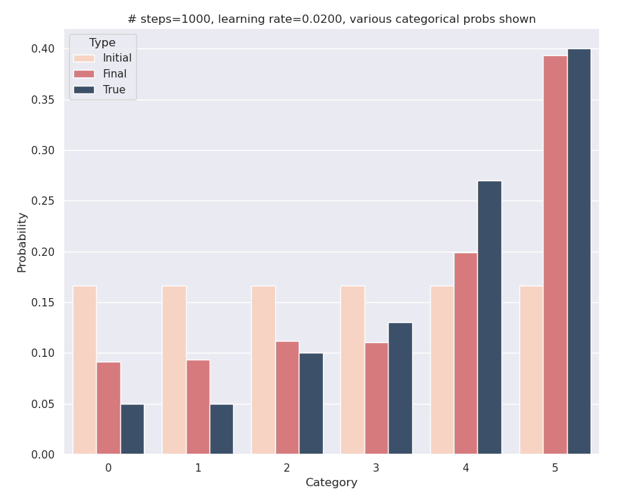
    demo()

Here are the results: although we start with equal logits, through the gradient descent process, we’ve managed to learn logits whose corresponding probabilities are close to the true values. Mission accomplished!

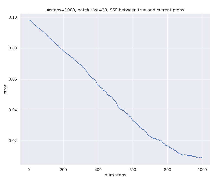
And here’s the SSE comparing the learned probabilities at any time and true probabilities look like:

References

1. McFadden, D. (1974). Conditional logit analysis of qualitative choice behavior. In P. Zarembka (Ed.), Frontiers in Econometrics (pp. 105–142). Academic press.
2. Jang, E., Gu, S., & Poole, B. (2017). Categorical Reparameterization with Gumbel-Softmax. International Conference on Learning Representations. https://openreview.net/forum?id=rkE3y85ee
3. Maddison, C. J., Mnih, A., & Teh, Y. W. (2017). The Concrete Distribution: A Continuous Relaxation of Discrete Random Variables. International Conference on Learning Representations. https://openreview.net/forum?id=S1jE5L5gl
4. Huijben, I. A. M., Kool, W., Paulus, M. B., & van Sloun, R. J. G. (2023). A Review of the Gumbel-max Trick and its Extensions for Discrete Stochasticity in Machine Learning. IEEE Transactions on Pattern Analysis and Machine Intelligence, 45(2), 1353–1371. https://doi.org/10.1109/TPAMI.2022.3157042
5. Kool, W., van Hoof, H., & Welling, M. (2019). Stochastic Beams and Where to Find Them: The Gumbel-Top-k Trick for Sampling Sequences Without Replacement. CoRR, abs/1903.06059. http://arxiv.org/abs/1903.06059