Jensen's Inequality - A Visual Intuition
Jensen’s inequality finds widespread application in mathematical proofs. I am fond of a particular intuitive explanation of it, which doesn’t seem to be very popular. I will try to present it in brief here.
I am not sure when this argument originated, but Google does turn up a paper (Needham, 1993). Even if this is not the source, it is a good reference. On a related note, the author of the paper, Tristan Needham, has the very well-reviewed book “Visual Complex Analysis” to his credit.
For the record, Wikipedia states one version in this way:
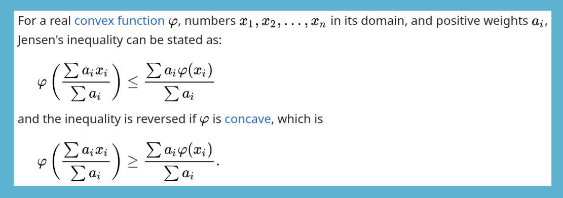
Jensen's Inequality, as on Wikipedia.
But don’t read too much into this yet; we’ll discover this form along the way. This is going to sound surprising but let’s start with the idea of the center of mass (CM).
Center of Mass
For our purposes, we can think of the center of mass of an object as that one point where you could hold up an object. Easy to intuit and easily shown with pictures. Below, you see the objects - a toy bird and a baseball bat - held up and balanced at their CM.

We wouldn’t be looking at the CMs of bodies like the toy bird or a baseball bat, but of groups of disconnected masses, like in the figure on the left below; here, a mass is represented by a circle, where its size corresponds to its mass. The CM is shown with a red square. If the disconnected-ness of the masses seems confusing, you could assume that the masses are affixed to a Plexiglas sheet of negligible weight, as shown on the right. Again, the intuition for the CM is that you can hold up this system and balance it at its location.
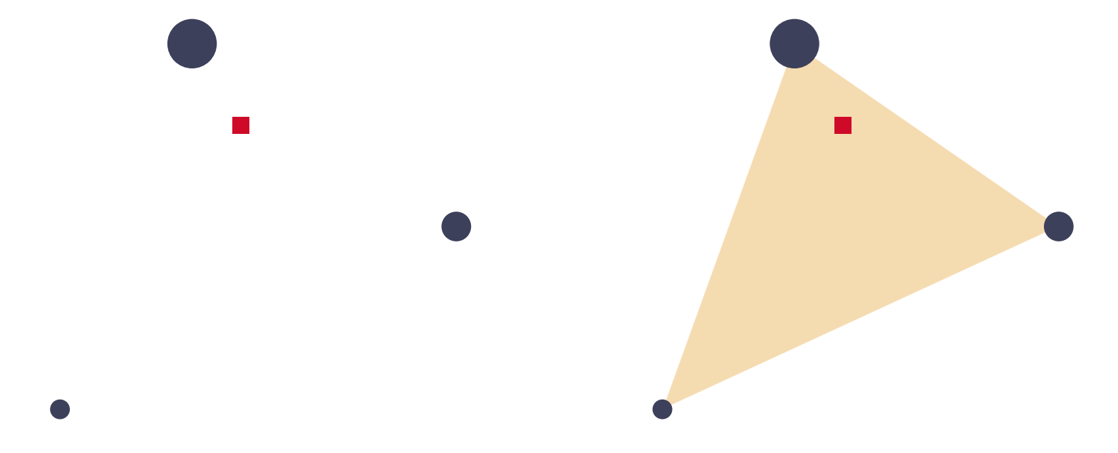
CM for some masses shown with a red square.
Let’s look at some more shapes - just to nail down the intuition. Here are some more mass placements and their CMs.

Some more mass distributions and their CMs.
The key takeaway - which might seem silly because it’s obvious to our physical intuition - should be that the CM always lies within the convex hull of the masses. There are great descriptions of convex hull online of course, but a description I like is: Think of the given points as locations of nails driven into a board. If you now were to snap a rubber band around these nails, the shape it ends up with is the convex hull. Let’s look at the masses above again - now with the convex hull also shown.
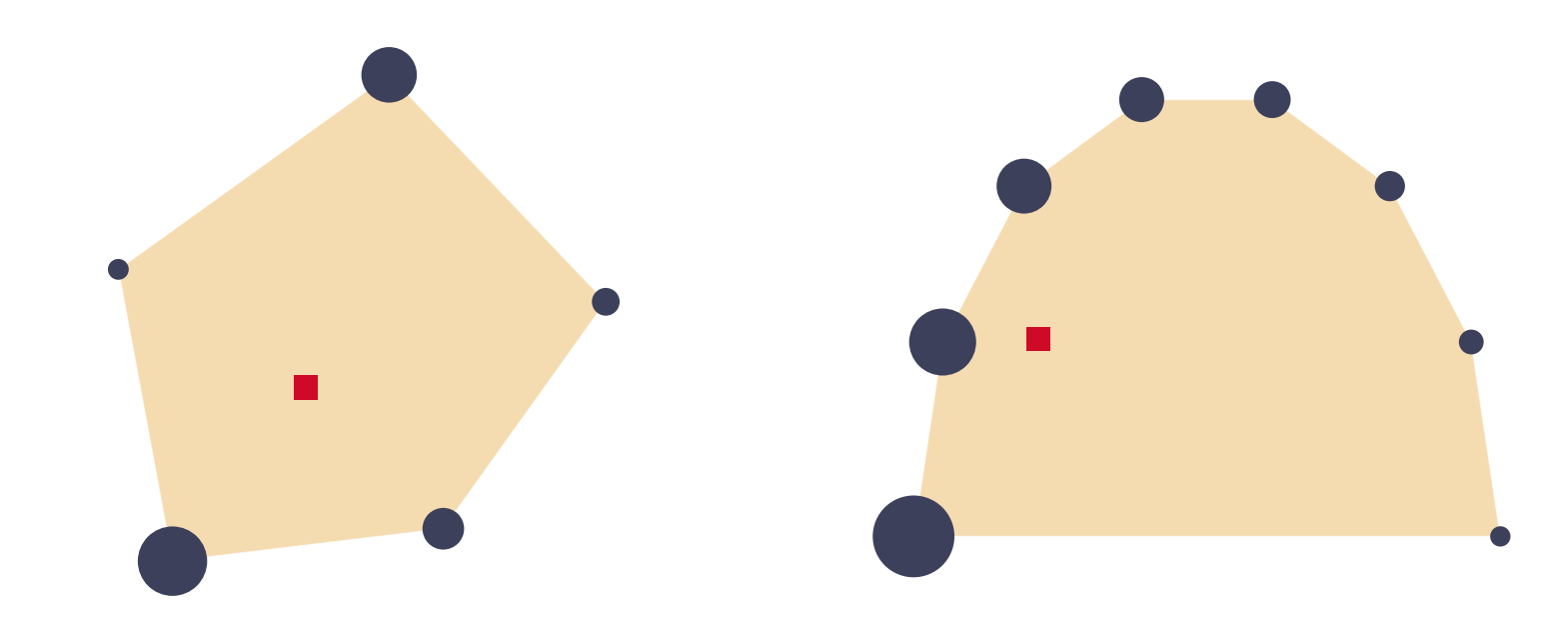
The CM always lies on the convex hull. Because, remember, you need to be able to physically hold up the system at this point!
Jensen’s Inequality
We now know enough to understand the inequality. Let’s first consider a concave curve \(f\) - the green line in the figure below. Assume we have placed four masses on it, as if we were stringing beads (the masses) with the curve. The masses and their locations are labeled: \(m_i, (x_i, y_i)\). Their CM is again shown with a red square; we’ll denote its coordinates as \((x_{CM}, y_{CM})\). As you might have come to expect, this is within the convex hull, which, importantly, itself is under the curve \(f\). Now consider the square with the red outline right above it - its y-coordinate is \(f(x_{CM})\). For a concave curve, this is greater than \(y_{CM}\), i.e., \(y_{CM} \leq f(x_{CM})\). Kind of obvious, isn’t it? Well that’s the inequality.
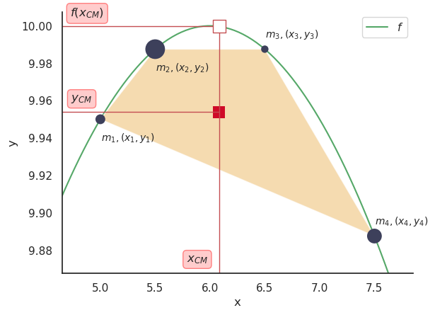
Finally: Jensen's Inequality!
Let’s write that down in symbols, starting with the familiar expressions for computing the CM’s coordinates:
\[\begin{aligned} x_{CM} = \frac{\sum_i m_i x_i}{\sum_i m_i}, \;\; y_{CM} = \frac{\sum_i m_i y_i}{\sum_i m_i} \end{aligned}\]Jensen’s inequality states that \(y_{CM} \leq f(x_{CM})\). The equality case occurs for some cases such as when all the masses have the same location. Substituting:
\[\begin{aligned} \frac{\sum_i m_i y_i}{\sum_i m_i} \leq f\Big(\frac{\sum_i m_i x_i}{\sum_i m_i}\Big) \end{aligned}\]Note that \(y_i = f(x_i)\), since the masses are on the curve \(f\). Let’s make this substitution as well:
\[\begin{aligned} \frac{\sum_i m_i f(x_i)}{\sum_i m_i} \leq f\Big(\frac{\sum_i m_i x_i}{\sum_i m_i}\Big) \end{aligned}\]This matches the wikipedia expression for the concave function we saw above. If we want to make the expression concise, we can use mass fractions, i.e., let \(a_i = m_i/\sum_j m_j\). Then the inequality may be written as:
\[\begin{aligned} \sum_i a_i f(x_i) \leq f\Big(\sum_i a_i x_i \Big) \end{aligned}\]For a convex curve, the sign of the inequality is reversed, i.e., \(y_{CM} \geq f(x_{CM})\), and we instead have:
\[\begin{aligned} \sum_i a_i f(x_i) \geq f(\sum_i a_i x_i) \end{aligned}\]References
- Needham, T. (1993). A Visual Explanation of Jensen’s Inequality. American Mathematical Monthly, 100. https://doi.org/10.2307/2324783